How LLMs Actually Work
You paste a stack trace into ChatGPT. Thirty seconds later, it explains the root cause, suggests a fix, and even warns you about an edge case you hadn’t considered. It reads like a reply from a senior engineer who’s debugged this exact problem before.
But what actually happened under the hood? The model predicted one token, then another, then another — each time picking the most plausible next piece of text given everything before it. That’s the core mechanism. Whether something deeper is happening inside — whether the model is “reasoning” in some meaningful sense — is an active research question. But the visible process is next-token prediction, and understanding how that works is what this post is about.
But “it just predicts the next token” is a bit like saying “a CPU just flips bits.” It’s true and it tells you nothing. This post is the version I wish I’d had — what actually happens under the hood, step by step, explained for people who write code for a living.
The pipeline at a glance
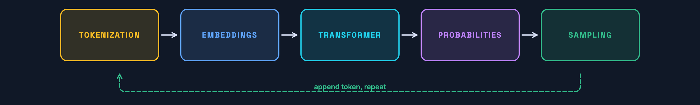
Every time a model generates a single token, this entire sequence runs:
- Tokenize the input text into integer IDs
- Embed each token as a high-dimensional vector
- Run through N transformer layers (attention + feedforward network)
- Score every token in the vocabulary as a possible next token
- Pick one from the probability distribution
- Append it to the input and repeat
At the architecture level, this is the entire loop — once per token. Some models add a separate reasoning phase with hidden tokens before visible output begins, but the underlying generation mechanism is the same.
Tokenization: compression before computation
The first thing that happens to your prompt is it gets chopped up. Not into words — into tokens.
A neural network operates on numbers, not characters. So before anything else, a tokenizer splits your input into chunks and assigns each one an integer ID.
The split isn’t always where you’d expect. Take a line of code:
def binary_search(arr, target):Paste it into OpenAI’s tokenizer and you’ll see it becomes 7 tokens: def, binary, _search, (arr, ,, target, ):.
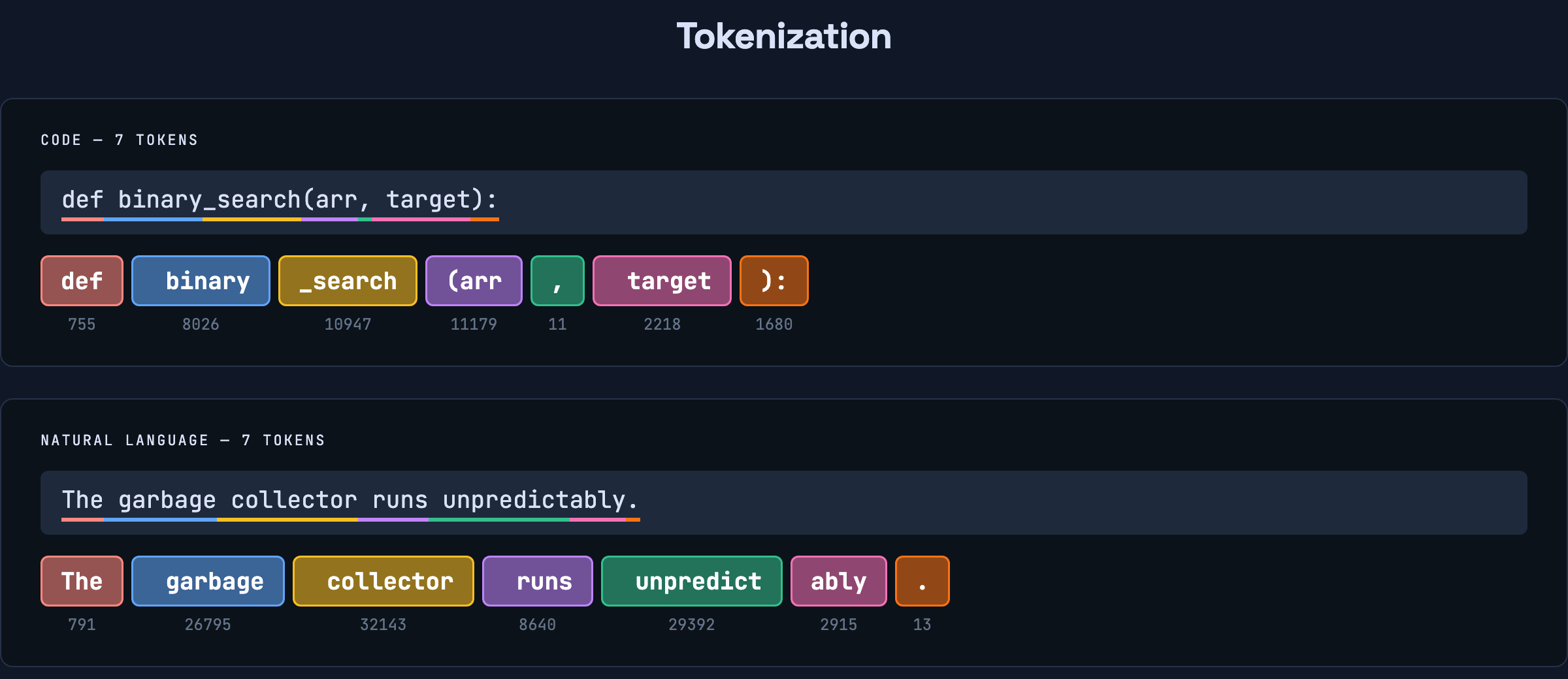
Not what you’d expect. The underscore in binary_search causes a split, but (arr gets merged into a single token because that pattern is common enough in training data. Same with ): — it’s one token, not two. The leading space before binary is part of that token, not a separate one. Even indentation in Python becomes tokens — whitespace matters to the model because it’s part of the input.
For natural language, the same thing happens. “Unpredictably” gets split into two pieces: unpredict and ably. The period is its own token. “Electromagnetic” splits into three: Elect, rom, agnetic. Meanwhile, “CPU” stays as one.
The tokenizer learns these splits from training data. Frequently occurring patterns get their own token. Rare patterns get decomposed into smaller, more common pieces. It’s a compression scheme — the same intuition behind Huffman coding, applied to text.
Different models use different tokenizers. The simplest approach is character-level: each character is a token, giving you a tiny vocabulary but very long sequences. In practice, most LLMs use subword tokenizers that find a middle ground. OpenAI uses tiktoken (Byte Pair Encoding), while many Google and open-source models use SentencePiece, a framework that can implement both BPE and unigram tokenization. They produce different splits and different vocabularies — GPT-4’s tokenizer has ~100K tokens, while a byte-level tokenizer starts with just 256 base symbols. The tradeoff is always the same: larger vocabulary means shorter sequences but a bigger embedding table.
This has practical consequences you’ve bumped into. API pricing is per token, not per word. Context windows are measured in tokens. A rough rule: one token is about three-quarters of a word in English. So a 128K-token context window holds roughly 96K words — but for code, the ratio is worse because of all the punctuation and whitespace tokens.
Try it yourself: Paste any text into OpenAI’s tokenizer and watch how it splits. Try code vs prose — you’ll see code uses more tokens per line than you’d expect.
After tokenization, your prompt is a sequence of integers. Our def binary_search(arr, target): becomes:
[755, 8026, 10947, 11179, 11, 2218, 1680]
That’s it. That’s what the model actually sees. def is 755. target is 2218. , is 11. These numbers carry no meaning on their own — 755 doesn’t encode anything about function definitions. It’s just a lookup index. The model needs something with structure.
Embeddings: giving tokens a location in meaning-space
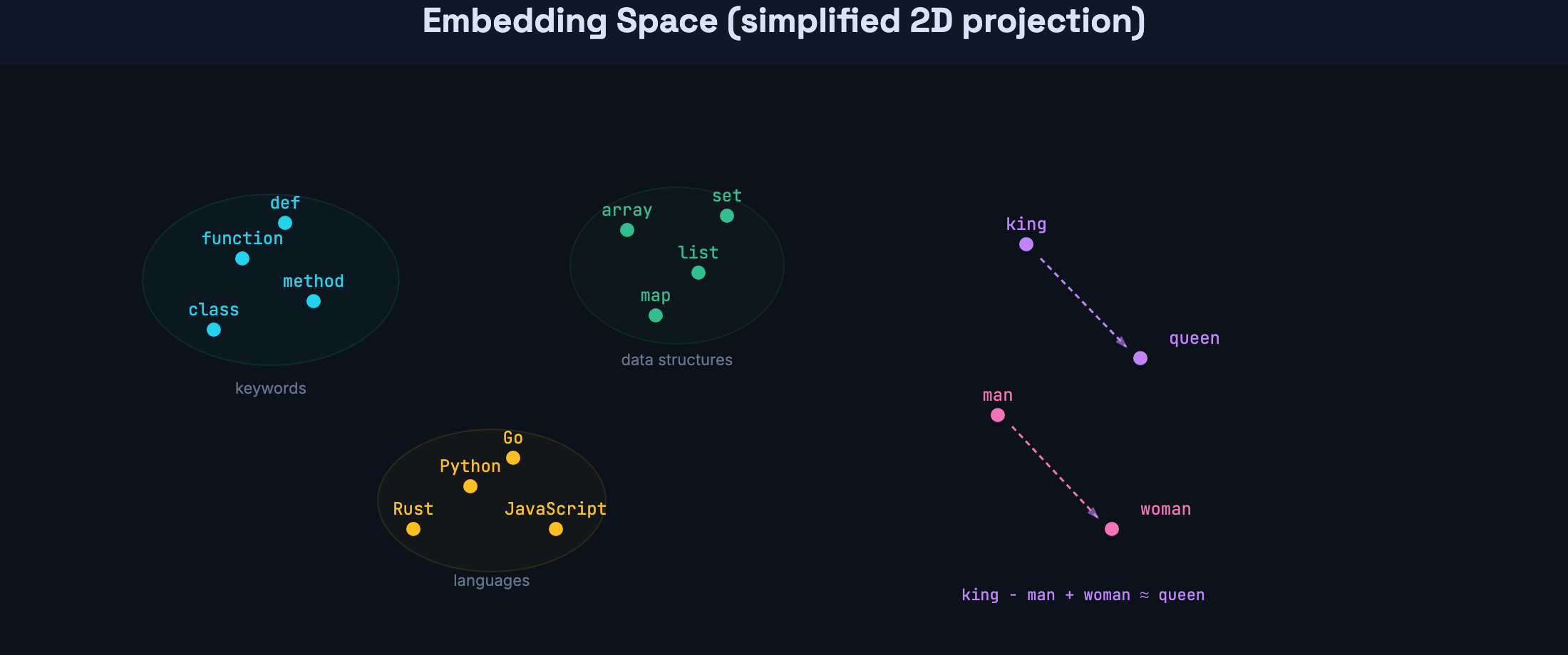
Each token ID gets mapped to a vector — a long list of floating-point numbers. GPT-3 uses vectors with over 12,000 dimensions. You can think of each vector as coordinates in a high-dimensional space where proximity encodes similarity.
This isn’t a metaphor. The geometry is real and measurable. After training, tokens that appear in similar contexts end up near each other in this space. “function” is near “method.” “array” is near “list.” “Python” is near “JavaScript” — not because anyone defined that relationship, but because they appear in similar contexts across the training data.
The classic demonstration is vector arithmetic: take the vector for “king,” subtract “man,” add “woman,” and you land near “queen.” That relationship was never programmed — it emerged from patterns in the training data.
These embedding vectors are what flow into the transformer — the neural network at the core of every LLM. From this point forward, everything the model does is operations on these vectors: comparing them, mixing them, transforming them. Raw text is gone. It’s all geometry now.
But embeddings alone have a problem. The token “Rust” gets the same initial vector whether it appears in “Rust’s borrow checker” or “rust formed on the iron gate.” Same for “class” — CSS selector, Python keyword, or college lecture? Same token, same ID, same starting embedding. The actual meaning depends entirely on the surrounding tokens. Resolving that ambiguity — figuring out which “Rust” or “class” this is — is the job of attention, which we’ll get to shortly.
Why the transformer exists: the sequential bottleneck
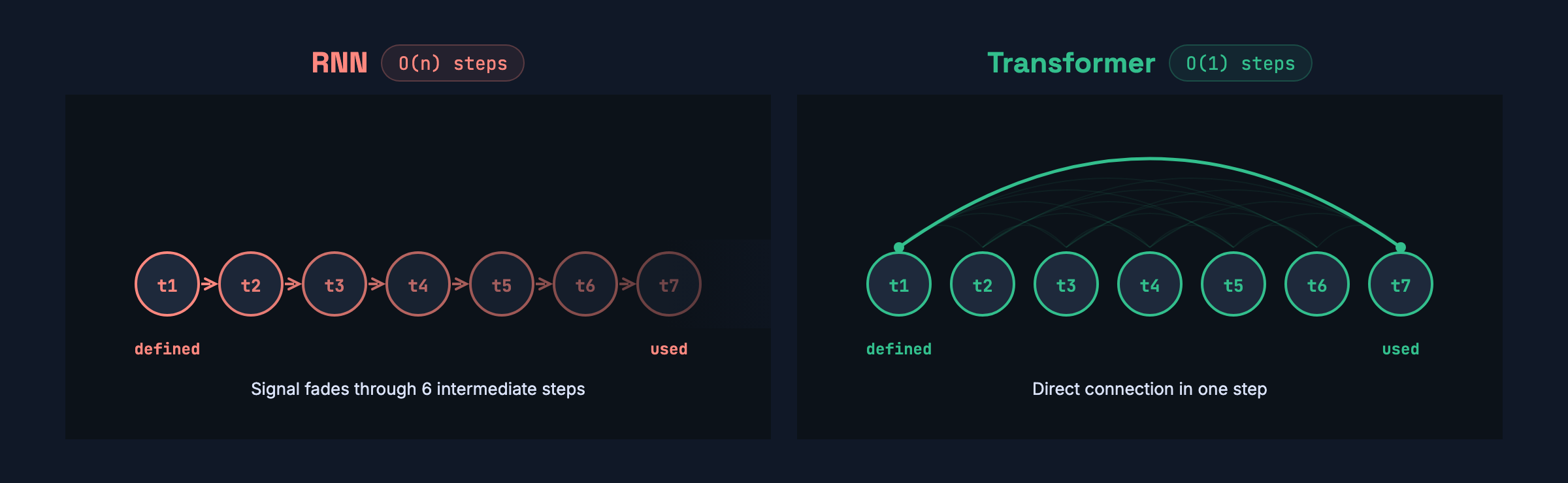
Before 2017, the go-to architecture for language was the recurrent neural network. RNNs read a sequence one token at a time, left to right, carrying a hidden state forward like a running summary.
This worked, but it had a fundamental limitation: it was sequential. Processing token 50 required finishing tokens 1 through 49 first. You couldn’t split the work across a GPU’s thousands of cores because each step depended on the previous one.
And there was a second problem. Information leaked out over distance. At each step, the RNN compresses everything it’s seen into a single fixed-size vector — think of it like a game of telephone. Token 1 whispers its information to token 2, which mixes it with its own and whispers the combined result to token 3, and so on. By token 500, the original message from token 1 has been mixed, compressed, and overwritten 499 times. The vector has finite capacity — it can’t faithfully preserve every detail from every previous token. New information pushes out old information.
If a variable used on line 47 was defined on line 3, the RNN has to hope that definition’s signal survived 44 rounds of this compression. Often it didn’t.
The transformer was designed to eliminate both of these constraints. It’s still a neural network — it has weights, it learns from data through backpropagation — but it’s wired up in a fundamentally different way. Instead of processing tokens sequentially, it processes them all at once using a mechanism called attention.
Attention: direct connections between every token
The core idea is deceptively simple: instead of passing information through a chain, let every token directly look at every previous token in one step. In modern decoder-only models like GPT and Claude, each token attends to everything before it — never future tokens. We’ll get to why shortly.
For each position, the model computes a relevance score against every other position in the sequence. High score means “this other token is important for understanding me.” These scores become weights, and the model creates a weighted mix of information from the most relevant positions.
Here’s where it gets concrete for code. Consider:
user = repo.find(user_id)
# ... 40 lines of other logic ...
return user.name
When the model processes user.name, it needs to know what user is. With attention, it directly looks back at user = repo.find(user_id) — regardless of how many lines separate them. It doesn’t matter if there are 5 lines or 500 lines in between. The path length is one step.
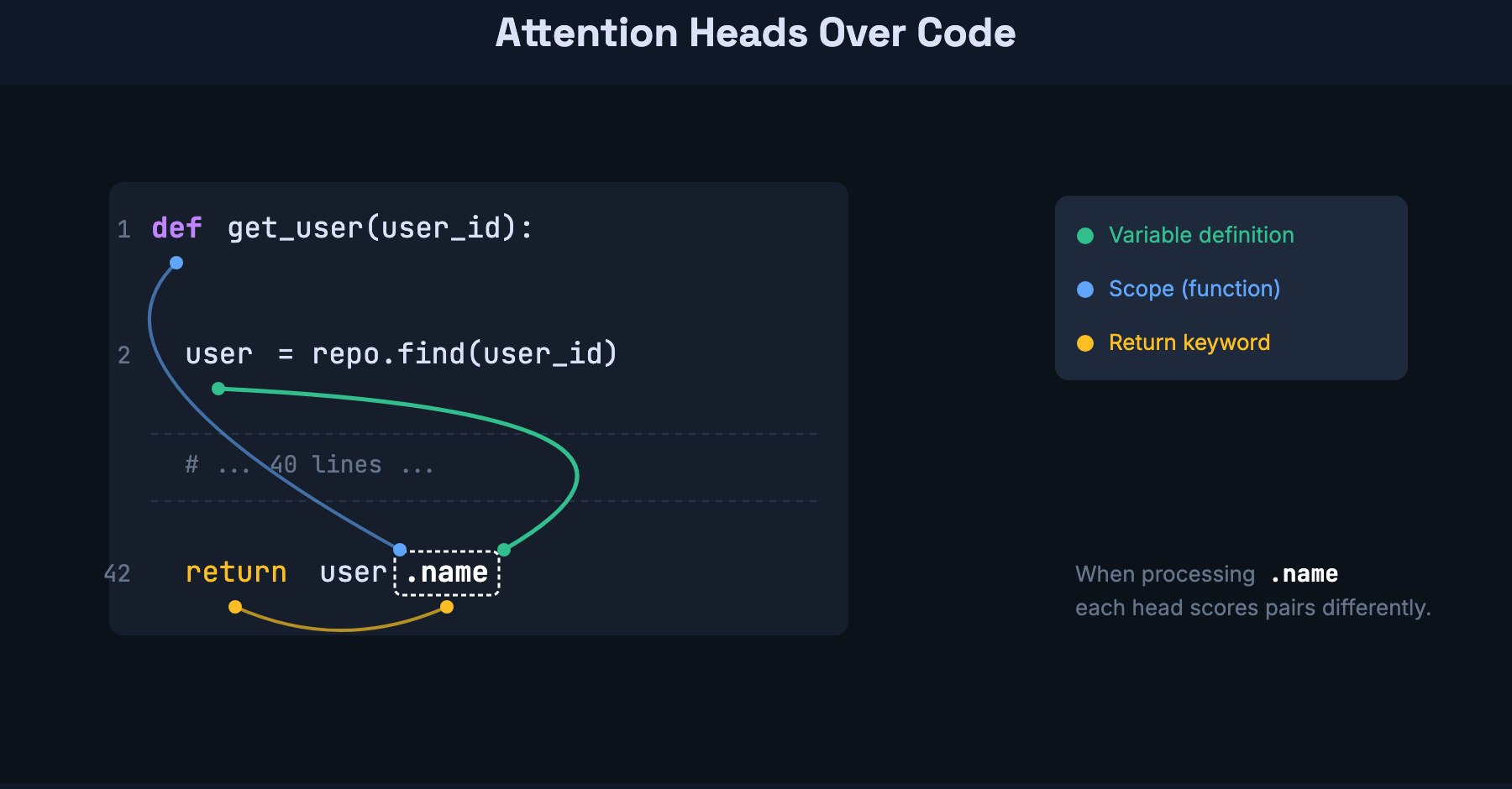
This is where code benefits even more than prose. Code has explicit long-range dependencies: a variable defined at the top of a function gets used at the bottom. An import statement at line 1 determines which methods are available at line 200. A function signature defines the contract that call sites rely on. These are all cases where attention’s O(1) path length — the ability to look anywhere in one step — pays off directly.
That’s attention at its simplest: every token can see every other token, in one step. Now let’s look at how the transformer actually implements this.
Inside the transformer: Q/K/V and multi-head attention
To compute those relevance scores, each token’s embedding gets transformed into three separate vectors through three learned weight matrices:
- Query (via W_Q) — “what am I looking for?”
- Key (via W_K) — “what do I have to offer?”
- Value (via W_V) — “what information do I carry?”
Each matrix compresses the full embedding — 12,288 dimensions in GPT-3 — down to a smaller vector of 128 dimensions. So every token in the sequence gets a query, a key, and a value, all 128-dim vectors produced by multiplying the token’s embedding by the corresponding weight matrix.
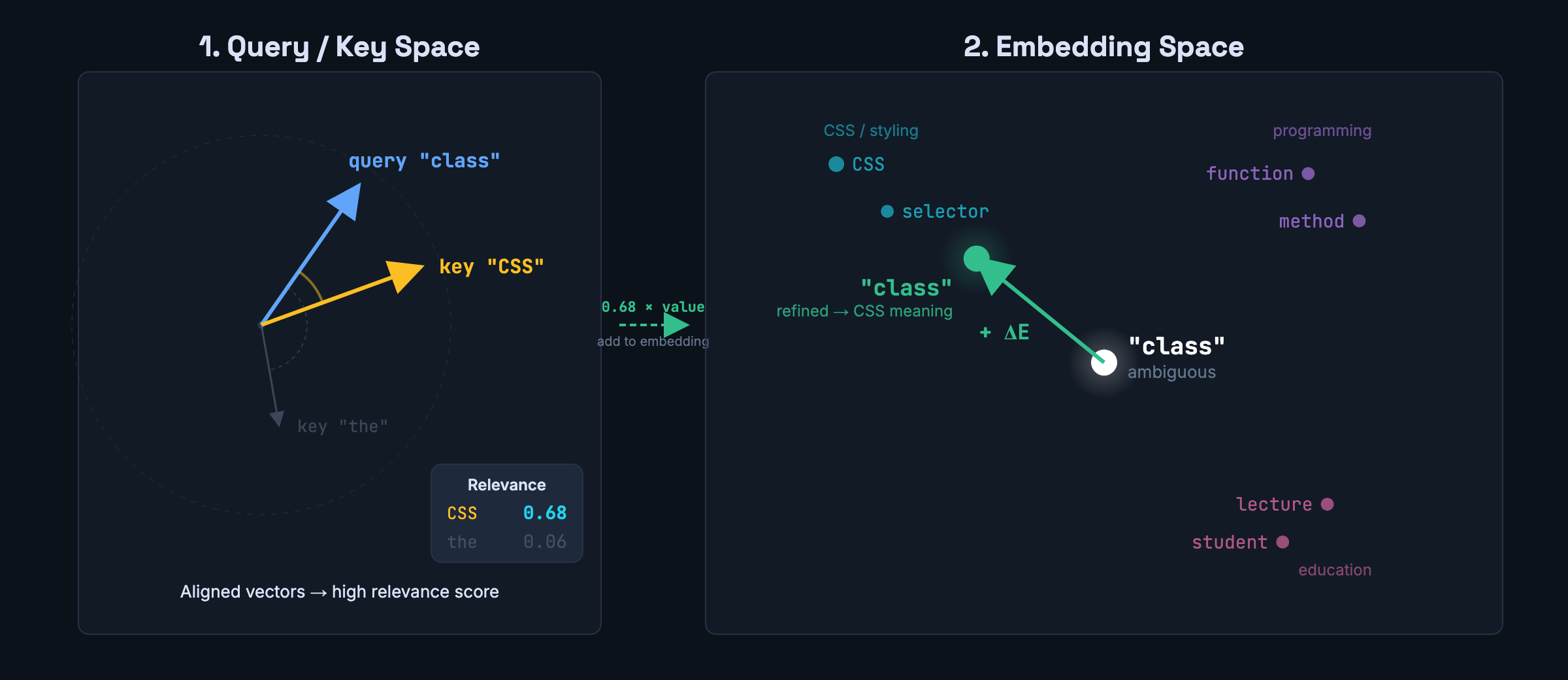
The relevance scores come from dot products between queries and keys. Take one token’s query vector and dot it with another token’s key vector — two 128-dim vectors produce a single number. High number means “this token is relevant to me.” Do this for every pair and you get a grid of scores across the full sequence. These dot products are divided by the square root of the key dimension to keep them from growing too large — without that, softmax would concentrate all weight on one token.
But the scores are just routing — they decide how much of each token’s information to pull in. The actual information being moved is the value vectors. Each value vector gets multiplied by its relevance score, and the results are summed into a single change vector. That change vector gets projected back up to the full embedding size and added to the original embedding. The token’s representation is now refined by context.
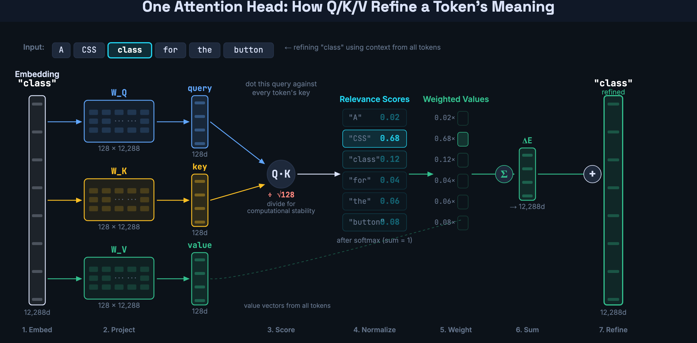
This is the complete attention operation for one head: compress embeddings into queries, keys, and values. Use queries and keys to compute relevance. Use relevance to weight the values. Add the weighted sum back to the embedding.
Geometrically, you can see what this does to a token’s position in embedding space. Before attention, “class” sits in an ambiguous region — equally close to CSS styling, Python keywords, and classrooms. In the query/key space, the query vector for “class” aligns closely with the key vector for “CSS” — producing a high relevance score. That means the value vector from “CSS” gets weighted heavily, and when it’s added to the embedding, “class” physically moves toward the CSS/styling cluster. One attention step, one disambiguation.
But a single attention operation has one set of Q/K/V projections, which means it learns one kind of question to ask about every token pair. That’s limiting, because code (and language) has many different kinds of relationships happening at once.
So the transformer runs 8, 16, or more attention operations in parallel — each with its own learned Q/K/V projections. These are called attention heads. Each head asks a different question across all token pairs.
For example, when processing the token name in return user.name, every head computes scores between name and every other token in the sequence. But they score differently:
- A “variable tracking” head might give a high score to
name↔user(on line 1, where the object was defined) and low scores to everything else - A “scope” head might give a high score to
name↔def(the function this code lives in) and low scores to the variable tokens - A “return tracking” head might give a high score to
name↔returnand ignore the rest
Same token, same set of pairs, but each head highlights different connections. Their results get concatenated and mixed into a single richer representation.
Why do different heads ask different questions? Each one starts with different random weights. During training, gradient descent pushes them apart — redundant heads don’t help reduce prediction error, so training pressure drives each head toward a different specialization. The architecture doesn’t assign roles. It just provides independent channels and lets training figure out how to use them.
Counting parameters
The numbers make the architecture tangible. Let’s walk through GPT-3.
The query and key matrices are small. Each one maps a 12,288-dimensional embedding down to 128 dimensions — about 1.6 million parameters per matrix. Two matrices per head, straightforward.
The value side has a problem. The weighted sum of values needs to be added back to the original embedding, which means the output needs to be 12,288 dimensions — not 128. A direct 12,288 → 12,288 mapping would require about 150 million parameters per head. With 96 heads, that’s 14 billion parameters in a single layer — before you’ve even stacked any layers. The model would be enormous and impossible to train.
The solution: route through the small space. One matrix compresses 12,288 → 128, another expands 128 → 12,288. Two small matrices instead of one massive one. The total parameter cost is the same as Q and K — about 1.6 million each.
That gives each head four matrices of roughly 1.6 million parameters: Q, K, value-compress, value-expand. About 6.3 million per head. Multiply by 96 heads and you get roughly 600 million parameters per attention layer. Stack 96 layers and attention accounts for about 58 billion parameters — roughly a third of GPT-3’s 175 billion total.
The other two-thirds? The feedforward networks between attention layers. Attention routes information between tokens, but feedforward layers are where most of the model’s learned knowledge actually lives.
Here’s an interesting historical detail. The original 2017 transformer was built for translation, not chat. It had two halves:
- Encoder — reads the full input sentence and builds a rich representation of it. Think of it as the “understanding” side.
- Decoder — generates the output one token at a time, using the encoder’s representation as a reference. Think of it as the “generating” side.
Each half used attention differently:
- The encoder used unmasked self-attention — every English word can see every other English word. The full input is already known, so no masking needed.
- The decoder used masked self-attention — when generating the output word by word, each position can only look at positions before it. Future tokens don’t exist yet.
- Cross-attention bridged the two — the decoder attended to the encoder’s output, connecting the generation to the input.
Modern LLMs like GPT, Claude, and Llama don’t use this full architecture. They’re decoder-only — they dropped the encoder and cross-attention entirely. All that remains is masked self-attention: each token attends to all previous tokens, but never future ones.
So the transformer wasn’t designed for LLMs as we know them today. It was a translation architecture, and LLMs use only the decoder half. But that half — masked self-attention with multiple heads, stacked in layers — turned out to be enough.
Now here’s the number that explains why the transformer replaced the RNN:
- RNN path length: O(n). Token 1 reaching token 100 takes 99 sequential steps.
- Transformer path length: O(1). One step. Any token to any token.
That’s it. That’s why transformers won. A constant-time path between any two positions, fully parallelizable on GPUs. The 2017 paper trained the base model on 8 P100 GPUs in 12 hours — the larger model took 3.5 days — and noted this was a small fraction of the training cost of prior state-of-the-art systems.
Positional encoding: restoring the sense of order
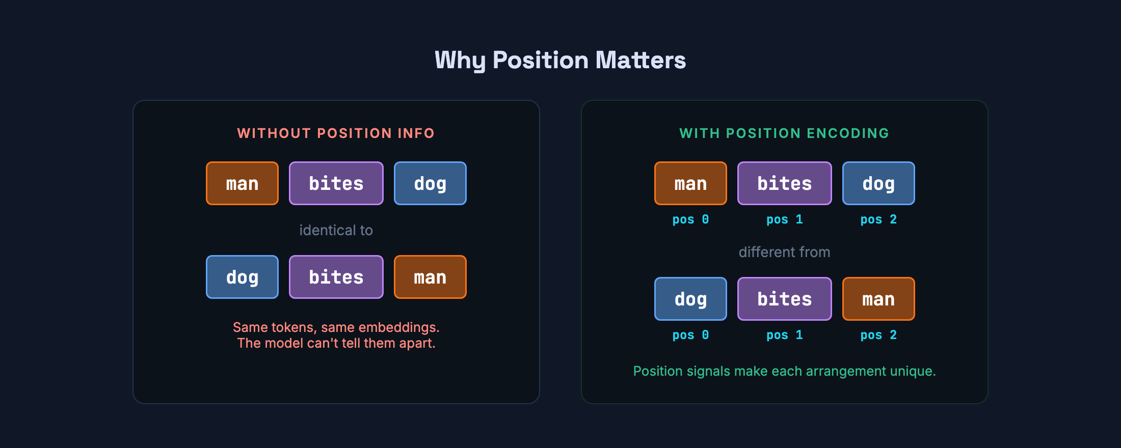
Attention has a trade-off. Because every token sees every other token simultaneously, it has no built-in sense of sequence. Shuffle the tokens and attention wouldn’t notice.
This matters. man bites dog and dog bites man use the exact same three tokens — man, bites, dog — but mean completely different things. Without position information, the model would see identical inputs for both. In code, the problem is even more obvious: x = 5; y = x + 1 is not the same as y = x + 1; x = 5.
To fix this, the transformer adds a position signal to each embedding before attention runs. The original 2017 paper uses overlapping sine and cosine waves at different frequencies — each position gets a unique fingerprint that the model can use to infer ordering and relative distance.
Modern LLMs have moved beyond fixed sinusoidal encodings. Most current models use rotary position embeddings (RoPE), which encode relative position directly into the attention computation rather than adding a separate signal to the embeddings. The intuition is the same — give the model a sense of order — but the implementation is more flexible and scales better to long contexts.
RNNs got sequence for free because they processed tokens in order. Transformers gave up that implicit ordering to gain parallelism, then added it back explicitly.
Layers: refining the representation
The transformer doesn’t run attention once and call it a day. It stacks identical layers — each consisting of an attention step followed by a feedforward network — and passes the data through all of them.
Attention moves information between tokens — it’s how one token learns about others. The feedforward network transforms information within each token — it’s a dense neural network that processes each token’s vector independently. Every layer has both: attention to route, feedforward to transform.
The original paper used 6 layers. GPT-3 uses 96. Each layer has its own set of attention heads with their own Q/K/V weights — so GPT-3 has 96 layers × 96 heads per layer = 9,216 separate attention operations. Each head operates on a smaller slice of the embedding (128 dimensions out of 12,288), so the total computation stays manageable. The model doesn’t need one layer to ask every possible question. It has 96 chances to run attention, each time on a more refined representation than the last.
Research shows a progression: early layers tend to encode syntactic structure and local patterns. Middle layers combine phrases and dependencies. Later layers encode more abstract properties like intent and long-range reasoning. The attention heads in layer 1 are asking questions about raw tokens. The heads in layer 90 are asking questions about meaning.
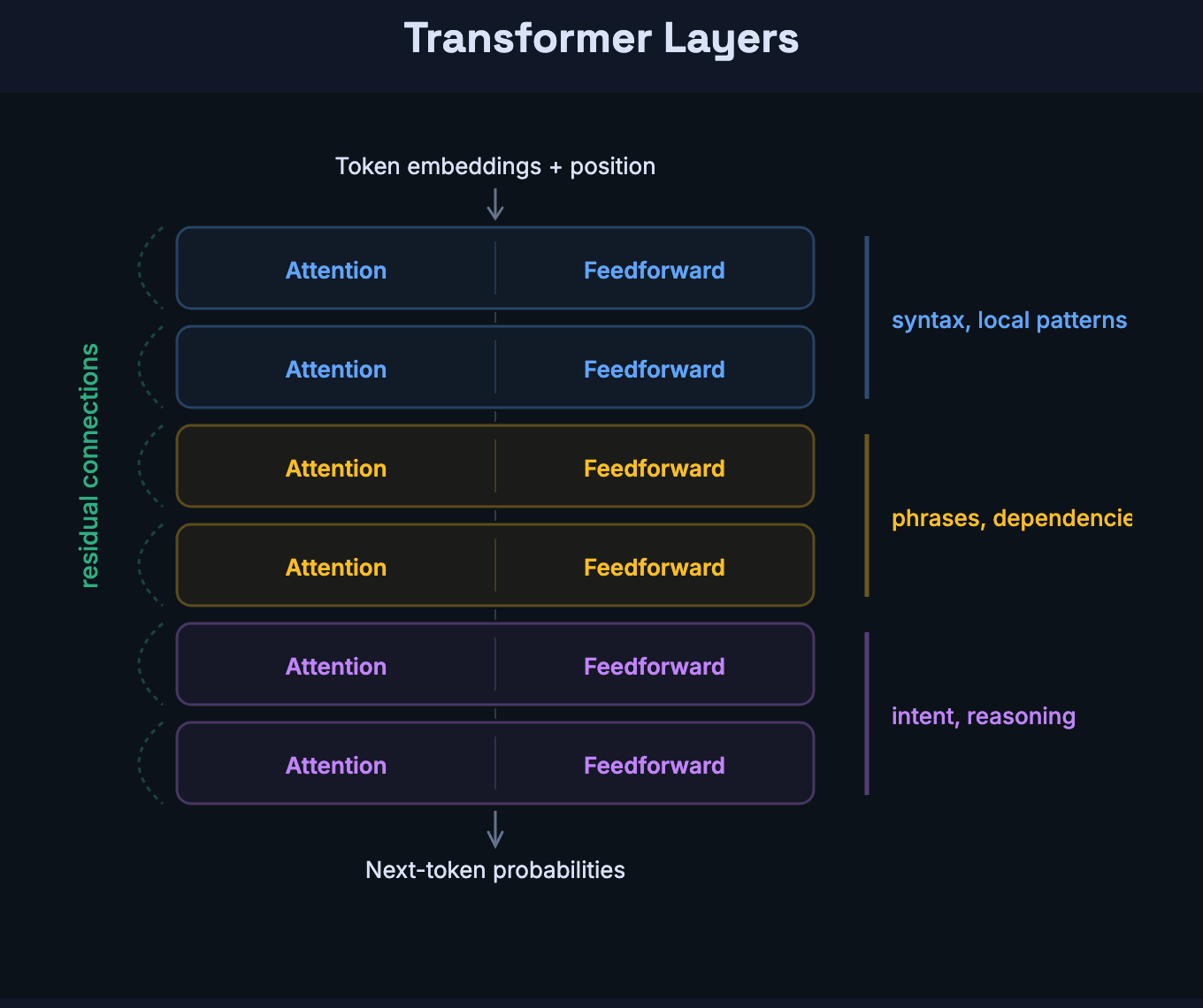
A key design choice makes this stacking work: residual connections. Each layer adds its output to its input rather than replacing it. Nothing from earlier layers is lost — just enriched. This matters for a practical reason: without residual connections, gradients can’t flow back through many layers during training. The signal degrades, and the network can’t learn. Residual connections create a shortcut path for gradients, keeping training stable even at 96 layers deep.
This is where the parameter count lives. To make the scale concrete: Karpathy’s nanoGPT trains a 10-million-parameter transformer on 300,000 tokens of Shakespeare in minutes. GPT-3 is 175 billion parameters trained on 300 billion tokens across thousands of GPUs. That’s roughly a millionfold increase in both model size and data — but the architecture is essentially identical. Same attention, same feedforward networks, same residual connections. Scale is the variable that changes everything.
From representation to prediction
After all the layers, the model has a deeply contextualized vector for the final position — one that encodes not just that token’s meaning, but its relationship to everything else in the input.
This vector gets projected into a score for every token in the vocabulary — over 100,000 of them. These raw scores are called logits — unnormalized numbers where higher means more plausible as the next token.
A function called softmax converts logits into a probability distribution: raise e to each logit, then divide by the sum so everything adds up to 1. For example, given the input “The server crashed because,” the model might produce:
the— 15%it— 12%of— 9%a— 7%there— 4%- … tens of thousands more tokens trailing off toward 0%
The model doesn’t have an answer. It has a distribution over every possible continuation. What you see as output is one sample from that distribution.
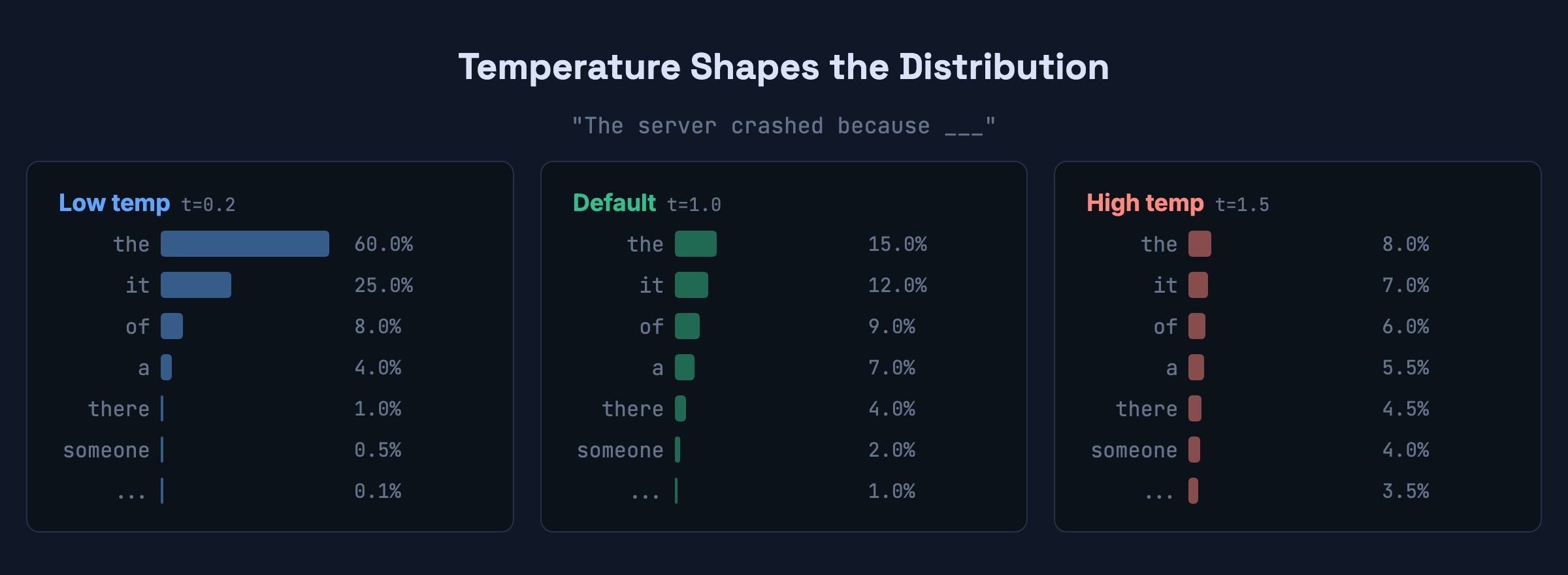
How the next token gets chosen
Given a probability distribution over 100,000+ options, the system picks one. The simplest strategy — always pick the highest probability — produces coherent but mechanical output. For our “The server crashed because” example, greedy decoding would always pick the (15%). Every time, same input, same output.
In practice, systems introduce controlled randomness. The main lever is temperature. It sharpens or flattens the distribution before sampling:
Low temperature (0.2) — the distribution sharpens. the might go from 15% to 60%. The model almost always picks the top candidate. Output is predictable and safe.
High temperature (1.5) — the distribution flattens. the drops to 8%, and tokens like there or someone get a real shot. Output is more varied but riskier. Push it too far and the signal-to-noise ratio collapses.
There’s also top-p sampling: only consider the smallest set of tokens whose combined probability exceeds a threshold. This adapts naturally — tight candidate set when the model is confident, wider when it’s uncertain.
If you’ve tuned these in an API call, you were directly shaping this selection. Low temperature for code generation where precision matters. Higher for brainstorming where variation helps.
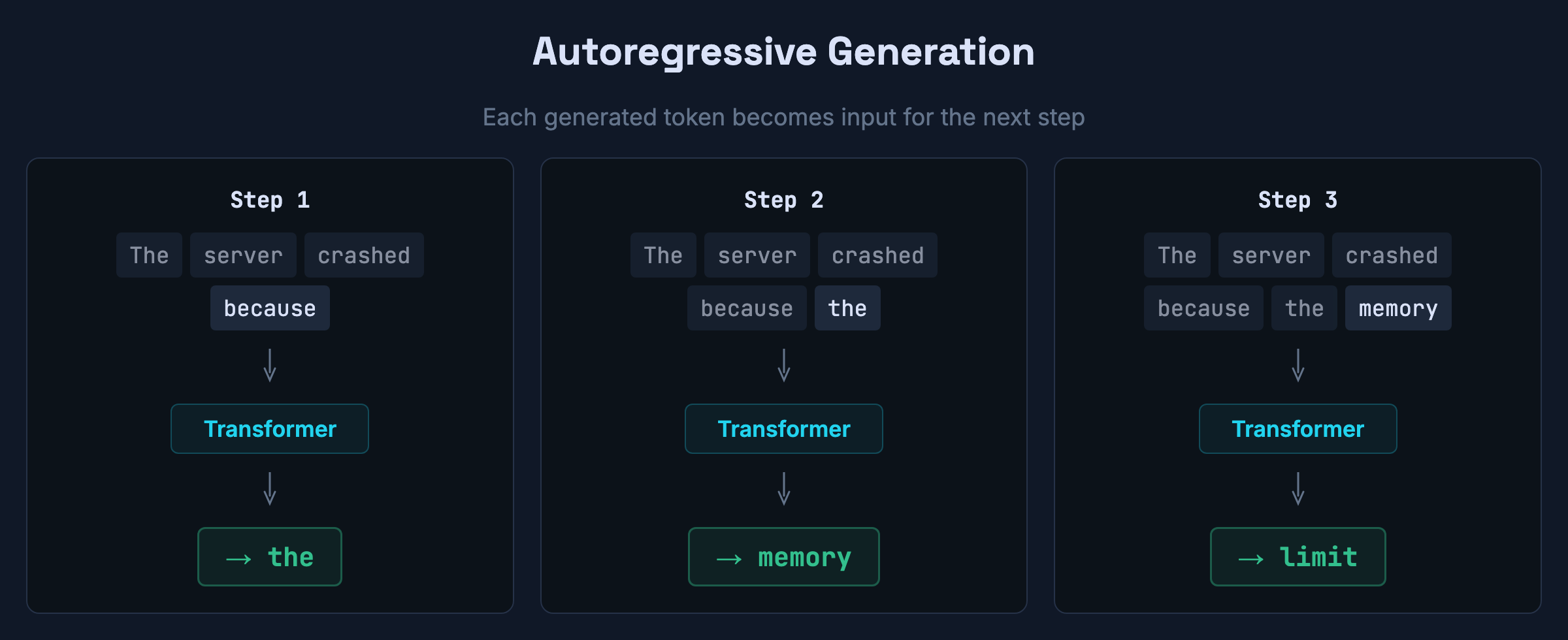
The generation loop in pseudocode:
tokens = tokenize(prompt)

while True:
    logits = model(tokens)
    next_token = sample(logits[-1], temperature=0.7, top_p=0.9)
    if next_token == END_OF_SEQUENCE or len(tokens) >= MAX_LENGTH:
        break
    tokens.append(next_token)
Generation stops when the model samples a special end-of-sequence token (meaning it considers the response complete) or when it hits a length limit — whichever comes first. That’s the entire process. One token at a time, appended, reprocessed.
One implementation detail worth knowing: in practice, models use KV caching — they store the key and value vectors from previous tokens so they don’t need to be recomputed on each step. This is why API pricing distinguishes between “input tokens” (computed once during prefill) and “output tokens” (generated one at a time). The pseudocode above is conceptually correct but the real implementation avoids redundant work.
Why prompting works
This pipeline also explains something that confuses a lot of developers: why prompting works at all.
A prompt doesn’t change the model’s weights. It changes the context flowing through those weights. Every token of your prompt is part of the input that attention operates over. Add a system prompt, a few examples, or a strict output schema, and you’ve changed the probability distribution of every subsequent token.
This is why few-shot prompting works. If you show the model three examples of input-output pairs before your actual question, you’ve loaded a pattern into the context window. Attention sees those examples and shifts its predictions to follow the same pattern. You’re not retraining the model. You’re conditioning it.
Prompting is programming by example. The context window is your runtime.
The context window is not memory
One more thing worth understanding: LLMs don’t have persistent memory.
What they have is a context window — a fixed-size buffer of tokens that attention can operate over. Anything inside the window can influence the output. Anything that’s fallen out of the window is gone, unless an external system retrieves it and injects it back.
This is why you can tell the model something at the start of a conversation and it “forgets” by the end of a long thread. It didn’t forget — the earlier tokens scrolled out of the window. Memory features in AI products aren’t a property of the model. They’re system design: something outside the model stores important context and re-injects it when needed.
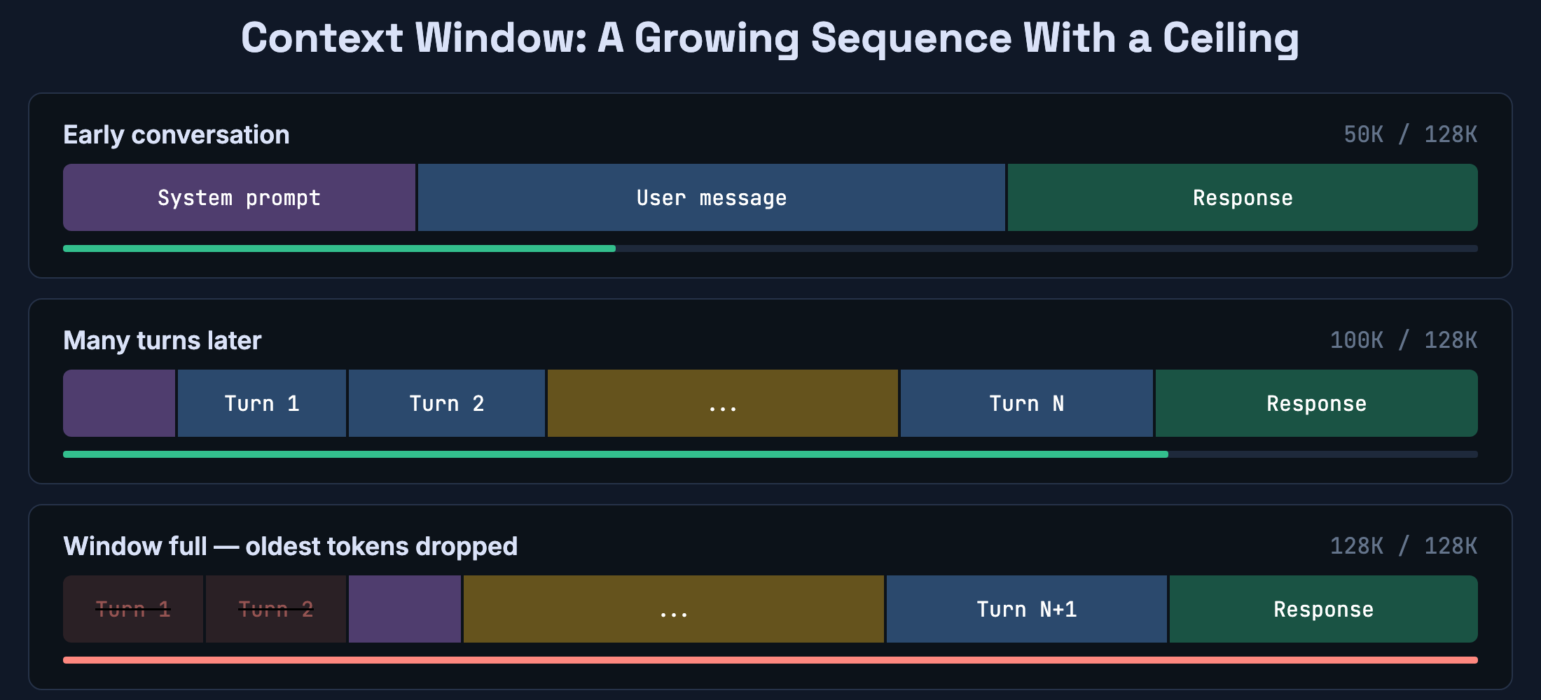
For developers building with LLMs, this is the most important architectural constraint to internalize. Your context window is finite. What goes into it is a design decision. Treat it like a cache, not like a brain.
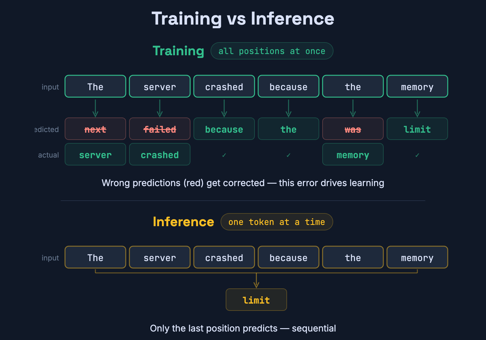
How the model learns
Everything above describes what happens at inference — when the model generates text. But how did the weights get to be the way they are?
Training is next-token prediction at massive scale. Take a sequence from the training data. Feed all but the last token into the model. Compare its prediction to the actual next token. The difference is the loss — a number that measures how wrong the prediction was.
Backpropagation then computes how each weight in the network contributed to that error and nudges every weight slightly to reduce it. Repeat this for trillions of tokens across a huge dataset of internet text, books, and code, and the model gradually compresses an enormous amount of statistical structure into its parameters: grammar, syntax, API patterns, factual regularities, even some reasoning-like behavior.
The key insight is that training is massively parallelizable. Unlike generation (which is sequential — one token at a time), training processes entire sequences at once. Every position in a training sequence produces a target, so a single forward pass generates many learning signals simultaneously. This is why training can leverage thousands of GPUs effectively, even though generation can’t.
From document completer to assistant
After pre-training, the model is not ChatGPT. It’s a document completer. Give it a question and it might respond with more questions — because that’s what internet documents look like. It might ignore your question and continue a news article. It babbles internet, not answers. It’s what Karpathy calls “totally unaligned.”
Turning a document completer into an assistant takes additional stages:
- Supervised fine-tuning (SFT) — train on thousands of question-answer pairs, so the model learns the format: question on top, helpful answer below.
- Reward modeling — human raters rank different model responses. A separate network learns to predict which responses humans prefer.
- Reinforcement learning (RLHF) — use the reward model to further tune the LLM so it generates responses that score highly on human preference. Newer approaches like Direct Preference Optimization skip the separate reward model entirely, but the goal is the same: align output with human preferences.
This fine-tuning data is typically not public. It’s a much smaller dataset than pre-training, but it dramatically changes the model’s behavior — from document completer to the assistant you interact with.
When you use an LLM through an API, you’re using the fine-tuned version. But under the hood, the same transformer architecture is running the same attention mechanism we’ve been discussing.
What this changes about how you work with LLMs
Once you understand the pipeline, certain behaviors stop being mysterious.
Why models sound confident about wrong things. The prediction step optimizes for plausible continuations, not truthful ones. A sentence that sounds authoritative and a sentence that’s actually correct often have similar probability distributions. The model has no fact-checker — it has a next-token predictor. Verification is your job.
Why longer contexts cost more. Standard attention computes scores between every pair of tokens. Double the context, quadruple the computation. In practice, production models use optimizations like FlashAttention and sparse attention patterns to reduce this cost, but the fundamental quadratic scaling of dense attention is why context windows have limits.
Why the same prompt gives different answers. Unless temperature is zero, sampling introduces randomness. The distribution is deterministic; the selection isn’t. The variation is a feature of how sampling works.
Why prompts are so sensitive to wording. Different tokens produce different attention patterns. Rephrasing your prompt changes which tokens attend to what, which changes the probability distribution, which changes the output. This isn’t a UX quirk — it’s a direct consequence of how the pipeline processes input.
The visible mechanism is simpler than most people expect. A pipeline converts text to numbers, refines those numbers through layers of attention, and predicts the next token from a probability distribution. Do that in a loop and you get output that’s coherent, useful, and occasionally remarkable. Whether the internal representations constitute something like understanding or reasoning is still debated — recent interpretability research suggests the answer may be more nuanced than “it’s just autocomplete.” But the architecture and decoding process are exactly what we’ve described.
Understanding the machinery doesn’t diminish what it produces. It just means you know what you’re building on.
References
- Attention Is All You Need — Vaswani et al., 2017. The original Transformer paper from Google that introduced the architecture behind every modern LLM.
- Large Language Models explained briefly — 3Blue1Brown’s visual walkthrough of transformers and attention.
- How Large Language Models Work — IBM Technology’s overview of LLM architecture and training.
- nanoGPT — Andrej Karpathy’s minimal GPT implementation for learning how transformers work in practice.
- OpenAI Tokenizer — Interactive tool to see how text gets split into tokens.
- tiktoken — OpenAI’s BPE tokenizer library.
- SentencePiece — Google’s subword tokenizer used in many open-source models.
Enjoyed this post?
I send an email every two weeks about computer science and software engineering. No fluff, no hype — just the mechanism behind the things we use every day.